Dir

Displays an object's normal direction and allows you to change it.

Steps:

• Select objects.

• Arrows show the normal direction.

• Move the cursor over the object to show a dynamic arrow for the direction.

• Click the mouse to flip (reverse) the normal direction.

Curve Options

Flip

Reverses the curve direction.

Surface Options

The arrow color for the u and v directions matches the construction plane x- and y-axis colors.

The draft angle for surfaces displays on the status bar.

UReverse/VReverse

Reverses the u- or v-direction.

SwapUV 

Swaps the u-and v-directions.

Flip

Reverses the surface direction.

Note: Closed polysurfaces cannot have their normal direction facing toward the interior of the object.

Flip

Reverses the object's normal direction.

Steps:

• Select objects.

• The command line reports the number of objects flipped.

Notes

• Closed polysurfaces cannot have their normal direction facing toward the interior of the object.

• The curve and surface directions affect the results of many surface creation commands and Boolean operations. If Boolean operations give unexpected results, such as a union instead of a difference, try flipping the normal direction of one or both of the surfaces.

Curvature

Analyzes the curvature at a point on a curve or surface.

Steps:

1. Select a curve.

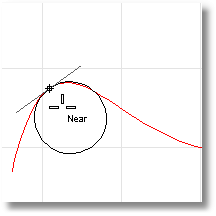
   The curvature radius of the curve at the marker will display in the status bar, and a black circle of that radius will display tangent to the curve at the marker. A white line tangent to the curve will also display.

2. Pick to mark the curvature with a circle, or press Esc to end the command.

To analyze surface curvature

1. Select a surface.

   As you move your cursor, two half-circles display and show you the minimum and maximum curvature at that point on the curve.

2. Pick a point on the surface.

   

   The following surface evaluation information displays in the command area:

   Surface curvature evaluation at parameter location
   3-D point
   3-D normal
   Maximum principal curvature
   Minimum principal curvature
   Gaussian curvature
   Mean curvature

Notes

• Every location on a smooth curve has a circle that best approximates the curve at that location.

• Every location on a smooth surface has two such circles. The circle with a biggest radius is always orthogonal to the circle with a smallest radius.

• The principal curvatures are inverse of the radii of the arcs.

• The Gaussian curvature is positive when both half circles point the same way, negative when the circles point opposite ways, and zero if one of the half circles degenerates into a line.

Options

MarkCurvature

If Yes, places a point object and the curvature circle or half circles at the evaluated point on a curve.

Gives permanent feedback when the radius of curvature is infinite (curvature is zero, the curve is locally flat, for example at inflection points where the curve bulge changes from one side to the other) and cannot be evaluated. This does not automate finding the inflection points, but it makes it possible to mark them manually.

CurvatureGraph

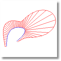
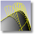
Turns curvature graph display on.

Steps:

• Select curves or surfaces.

• A graph showing curvature appears on the selected curves, and the Curvature Graph dialog box appears.

  Adjust the length, frequency, color, u- and v-direction display of the curvature indicators using the controls in the Curvature Graph dialog box.

  Even when other commands are started, the curvature graphs and the Curvature Graph dialog box persist until you turn them off.

Curve Analysis

Tangent

Even though the curve spans are tangent to one another, the curvature graph suddenly changes from one value to a different value. The spans of a degree 2 curve are G1, or tangent only. They are not curvature continuous.

Curvature Continuous

There are no jumps in the curvature graph. The curvature graph of the first span connects end-to-end with the curvature graph of the second span. This curve is curvature continuous (G2) across its spans because its curvature does not suddenly go from one value to another value. However, the curvature graph of the first span does not progress at the same rate as the graph of the second span. So even though the curvature stays the same, the rate of curvature suddenly changes.

To better grasp this concept, play with the Curvature command and observe the osculating circle as it travels along curves.

Notes

• On surfaces the curvature hairs only display at surface isoparametric curves. If the isoparametric curve display is turned off, curvature hairs display only at the surface boundary.

• At any location on a curve (except lines), there is a circle that most closely resembles the curve at that location. That is, it has the same tangent direction and the same rate of change of the tangent direction. The curvature displayed is a graph of (1/radius of that circle), but it is scaled by a factor set in the dialog box. If the graph changes smoothly, the curve is "smooth" or "fair." Jumps in the curvature graph indicate kinks or abrupt changes in the curve's derivatives.

Options

Display Scale

Sets the size of the graph hairs. Remember that the scale of the changes can be greatly exaggerated. The changes in curvature may be no thicker than a coat of paint. A Display scale setting of 100 means a 1:1 curvature scale.

Density

Sets the number of graph hairs.

Curve Hair color

Sets the graph hair color for curves.

Surface Hair color

Sets the graph hair color for surfaces.

U/V

Displays surface hairs in the u- or v-direction only.

Add Objects

Turn on curvature graph display for additional selected objects.

Remove Objects

Turn off curvature graph display for selected objects.

CurvatureGraphOff

Turns off curvature graph display for curves and surfaces.

CurvatureAnalysis

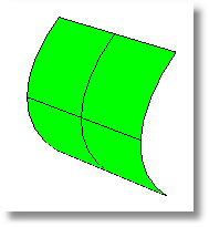
Displays false-color curvature analysis on surfaces.

These tools can be used to gain information about the type and amount of curvature on a surface. Gaussian and Mean curvature analysis can show if and where there may be anomalies in the curvature of a surface.

Unacceptably sudden changes like  bumps, dents, flat areas or ripples, or in general areas of curvature that are higher or lower than the surrounding surface can be located and corrected if needed.

Gaussian curvature display is helpful in deciding whether or not a surface can be developed into a flat pattern.

A smooth surface has two principal curvatures. The Gaussian curvature is a product of the principal curvatures. The Mean curvature is the average of the two principal curvatures.

Steps:

1. Select objects.

2. Set the style and range.

Options

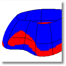
Gaussian

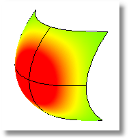
In the images below, red is assigned to a positive value of Gaussian curvature, green is assigned to zero Gaussian curvature, and blue to a negative value of Gaussian curvature.

Any points on the surface with curvature values between the ones you specify will display using the corresponding color. For example, points with a curvature value half way between the specified values will be green. Points on the surface that have curvature values beyond the red end of the range will be red and points with curvature values beyond the blue end of the range will be blue.

Results

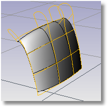
Positive curvature

A positive Gaussian curvature value means the surface is bowl-like.

Negative curvature

A negative value means the surface is saddle-like.

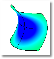
Zero curvature

A zero value means the surface is flat in at least one direction. (Planes, cylinders, and cones have zero Gaussian curvature).

If you know the value range of the curvature you are interested in analyzing, type those values in the edit boxes next to the red and blue portions of the "rainbow." The values you use for red should be different from the value you use for blue, but the value for red can be larger or smaller than the value for blue.

Options

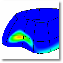
Mean

Displays the absolute value of the mean curvature. It is useful for finding areas of abrupt change in the surface curvature.

Max radius

This option is useful for flat spot detection. Set the value of blue to be rather high (10 >100 >1000) and of red to be close to infinity. Red areas in the model then indicate flat spots where the curvature is practically zero.

Min radius

If you are going to offset a surface at distance r or are going to mill a surface with a cutting ball of radius r, then any place on the surface that "curves" with a radius smaller than r will cause trouble.

In the case of an offset, you'll get a twisty mess that goes through itself. In the case of the mill, your cutting ball will remove material you want to keep.

In these cases you need to be able to answer the question, "Does this surface have any place where it bends too tightly?" The Min Radius option should help you answer this question.

Set RED = r set BLUE = 1.5 x r

You cannot offset/mill anywhere on the surface that is red. Blue areas should be safe. However, you should view areas from green to red with suspicion.

Auto Range

Using false color mapping, the CurvatureAnalysis command analyzes surface curvature. You have to map values to saturated computer colors. As a starting point, use Auto Range and then adjust the values to be symmetric but with magnitudes comparable to those selected by Auto Range.

The CurvatureAnalysis command attempts to remember the settings you used the last time you analyzed a surface. If you have dramatically changed the geometry of a surface or have switched to a new surface, these values may not be appropriate. In this case, you can use Auto Range to automatically compute a curvature value to color mapping that will result in a good color distribution.

Max Range

Choose this option if you want the maximum curvature to map to red and the minimum curvature mapped to blue. On surfaces with extreme curvature variation, this may result in a rather uninformative image.

Notes

• If, when you use the CurvatureAnalysis command, any selected object does not have a surface analysis mesh, an invisible mesh will be created based on the settings in the Polygon Mesh Options dialog box.

• The surface analysis meshes are saved in the Rhino files. These meshes can be large. The RefreshShade command and the Save geometry only option of the Save and SaveAs commands remove any existing surface analysis meshes.

• To properly analyze a freeform NURBS surface, the analysis commands generally require a detailed mesh.

CurvatureAnalysisOff

Closes the Curvature Analysis dialog box.

Gaussian and mean curvature

To understand Gaussian curvature of a point on a surface, you must first know what the curvature of curve is.

At any point on a curve in the plane, the line best approximating the curve that passes through this point is the tangent line. We can also find the best approximating circle that passes through this point and is tangent to the curve. The reciprocal of the radius of this circle is the curvature of the curve at this point.

The best approximating circle may lie either to the left of the curve, or to the right of the curve. If we care about this, then we establish a convention, such as giving the curvature positive sign if the circle lies to the left and negative sign if the circle lies to the right of the curve. This is known as signed curvature.

Normal section curvature is one generalization of curvature to surfaces. Given a point on the surface and a direction lying in the tangent plane of the surface at that point, the normal section curvature is computed by intersecting the surface with the plane spanned by the point, the normal to the surface at that point, and the direction. The normal section curvature is the signed curvature of this curve at the point of interest.

If we look at all directions in the tangent plane to the surface at our point, and we compute the normal section curvature in all these directions, then there will be a maximum value and a minimum value.

Principal curvatures

The principal curvatures of a surface at a point are the minimum and maximum of the normal curvatures at that point. (Normal curvatures are the curvatures of curves on the surface lying in planes including the tangent vector at the given point.) The principal curvatures are used to compute the Gaussian and Mean curvatures of the surface.

Gaussian curvature

The Gaussian curvature of a surface at a point is the product of the principal curvatures at that point. The tangent plane of any point with positive Gaussian curvature touches the surface at a single point, whereas the tangent plane of any point with negative Gaussian curvature cuts the surface. Any point with zero mean curvature has negative or zero Gaussian curvature.

Mean curvature

The Mean curvature of a surface at a point is one half the sum of the principal curvatures at that point. Any point with zero mean curvature has negative or zero Gaussian curvature.

Surfaces with zero mean curvature everywhere are minimal surfaces. Surfaces with constant mean curvature everywhere are often referred to as constant mean curvature (CMC) surfaces.

CMC surfaces have the same mean curvature everywhere on the surface.

Physical processes which can be modeled by CMC surfaces include the formation of soap bubbles, both free and attached to objects. A soap bubble, unlike a simple soap film, encloses a volume and exists in an equilibrium where slightly greater pressure inside the bubble is balanced by the area-minimizing forces of the bubble itself.

Minimal surfaces are the subset of CMC surfaces where the curvature is zero everywhere.

Physical processes which can be modeled by minimal surfaces include the formation of soap films spanning fixed objects, such as wire loops. A soap film is not distorted by air pressure (which is equal on both sides) and is free to minimize its area. This contrasts with a soap bubble, which encloses a fixed quantity of air and has unequal pressures on its inside and outside.

DraftAngleAnalysis

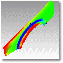
Turns false-color draft angle analysis on.

Steps:

1. Select objects.

2. In the Draft Angle dialog box, set the angle for the color display.

   The draft angle depends on the construction plane orientation. When the surface is vertical/perpendicular to the construction plane, the draft angle is zero. When the surface is parallel to the construction plane, the draft angle is 90 degrees.

   You can adjust the density of the mesh if the level of detail is not fine enough.

Notes

• If you set the minimum and maximum angle to the same value, all portions of the surface that exceed the angle will be red.

• 

• The pull direction for DraftAngleAnalysis is the z-axis of the construction plane that is in the active viewport when the command starts.

• The normal direction of the surface is the same as the pull direction of the mold. You can check this with the Dir command.

• Changing the construction plane before using DraftAngleAnalysis lets you define any direction as the pull direction.

DraftAngleAnalysisOff

Turns false-color draft angle analysis off.

Zebra

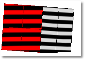
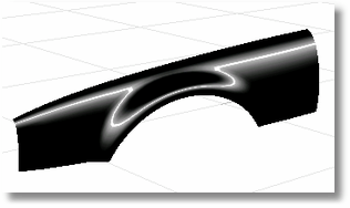
Maps stripes onto surfaces and meshes for analysis.

Steps:

• Set the stripe direction, size, and color.

• Set the stripe color to contrast with the base color of the object to see the zebra stripes.

  The first stage is to set the detail level for the analysis mesh. You can increase the density of the mesh if the level of detail is not fine enough.

  

The Zebra command is one of a series of visual surface analysis commands. These commands use NURBS surface evaluation and rendering techniques to help you visually analyze surface smoothness, curvature, and other important properties.

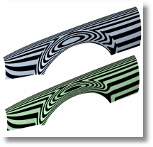
Interpreting the stripes

Position Only (G0)

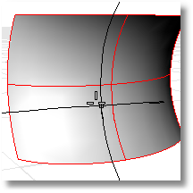
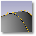
If the stripes have kinks or jump sideways as they cross the connection from one surface to the next, the surfaces touch, but have a kink or crease at the point where the zebra stripes jag. This indicates G0 (position only) continuity between the surfaces.

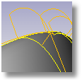
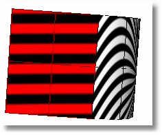
Tangent matches; curvature does not match (G1)

If the stripes line up as they cross the connection but turn sharply at the connection, the position and tangency between the surfaces match. This indicates G1 (position + tangency) continuity between the surfaces. Surfaces that are connected with the FilletSrf command display this behavior.

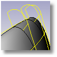
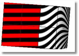
Position, curvature, and tangency match (G2)

If the stripes match and continue smoothly over the connection, this means that the position, tangency, and curvature between the surfaces match. This matching indicates G2 (position + tangency + curvature) continuity between the surfaces. Surfaces connected with the BlendSrf, MatchSrf, or NetworkSrf commands display this behavior. When you use surface edges as part of the curve network, the NetworkSrf options allow any of these connections.

If, when you use the Zebra command, the selected objects do not already have a surface analysis mesh, an invisible mesh will be created based on the settings in the Polygon Mesh Options dialog box.

The surface analysis meshes save in the Rhino files. These meshes can be large. The RefreshShade command and the Save geometry only option of the Save and SaveAs commands remove any existing surface analysis meshes.

To properly analyze a freeform NURBS surface, the analysis commands generally require a detailed mesh.

ZebraOff

Turns off Zebra analysis and closes the Zebra dialog box.

Steps:

• Close the Zebra Options dialog box.

EMap

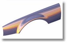
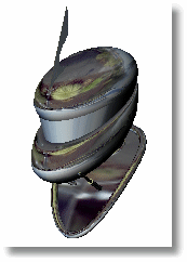
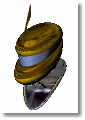
Turns on shaded environment mapping for surface analysis.

Steps:

1. Select the objects for environment mapping.

2. In the Environment Map Options dialog box, select a bitmap file to use for mapping.

Options

Blend with object render color

This blends the bitmap with the render color of the object, which lets you simulate different materials with the environment map. To simulate different materials, use a neutral colored bitmap and blend with the object render color.

Notes

• The EMap command is one of a series of visual surface analysis commands. These commands use NURBS surface evaluation and rendering techniques to help you visually analyze surface smoothness, curvature, and other important properties.

• If, when you use the EMap command, any selected object does not have a surface analysis mesh, an invisible mesh will be created based on the settings in the Polygon Mesh Options dialog box.

• The surface analysis meshes are saved in the Rhino files. These meshes can be large. Both the RefreshShade command and the Save geometry only option of the Save and SaveAs commands remove any existing surface analysis meshes.

  To properly analyze a freeform NURBS surface, the analysis commands generally require a detailed mesh.

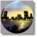
• Environment mapping is a rendering style that makes it look as though a scene is being reflected by a highly polished metal. There may be a few cases in which environment mapping actually shows a surface defect that can't be seen when you use Zebra and rotate the scene.

• 

Environment map images

Images for environment mapping are created by photographing a reflective sphere in various environments.

Manipulating a flat image to be round using a paint program does not work, for this procedure doesn't capture the whole environment. To better understand why, find something (anything) that's reflective and look at the reflections carefully. A chrome toaster, or some other approximately spherical object, will aid your understanding especially well.

As you look into the center of the object you will see yourself. But as you look toward the edge of the object (where the surface normal is almost perpendicular to the direction you are looking) you will see that the reflected object is almost exactly behind the object you are looking at. The result is that a reflective sphere shows a distorted view of the entire scene around it - in front of, beside, and behind the sphere. All reflective objects do the same.

A photograph, on the other hand, shows only a small portion of what is in front of the camera, which is not even close to a 360 degree view. You can use a fish-eye lens to get a closer approximation, but you still only get a 180 degree view at best.

There are some software programs that will take a series of panoramic photos (take them by putting your camera on a tripod and rotating the camera until you get shots of everything around the camera) and combine them into a spherical map.

EMapOff

Turns off environment map display.